API
The geolayerBDAP library consists of two classes:
rasterlayer (see rasterlayer) is the class dedicated to the display of raster datasets (.tif, .vrt, .nc, and all other raster formats managed by the GDAL library)
vectorlayer (see vectorlayer) is the class that enables the display of shapefiles, geopackage, POSTGIS queries and WKT strings on a ipyleaflet Map

rasterlayer
Display of raster datasets (.tif, .vrt, .nc, and all other formats managed by the GDAL library)
- class rasterlayer.rasterlayer(filepath='', band=1, epsg=4326, proj='', nodata=999999.0, identify_dict=None, identify_integer=False, identify_digits=6, identify_label='Value')
Raster datasets visualization. Class to display any type of raster dataset format managed by the GDAL library.
An instance of this class can be created using one of these class methods:
For Sentinel-2 L2A products, these class methods can be used:
To define the visual appearance of rasters, these methods can be used:
- classmethod single(filepath, band=1, epsg=None, proj='', nodata=None, identify_dict=None, identify_integer=False, identify_digits=6, identify_label='Value')
Single layer raster display.
- Parameters:
filepath (str) – File path of the raster to display.
band (int, optional) – Band number (from 1 to n) to display (default is 1).
epsg (int, optional) – EPSG code of the coordinate system to use (default is None which causes the reading of the info from the input file).
proj (str, optional) – Proj4 string of the coordinate system to use (default is the empty string). If a non-empty string is passed, the proj parameter has prevalence over the epsg code.
nodata (float, optional) – Value to be considered as absence of data (default is None, which causes the reading of the info from the input file).
identify_dict (dict, optional) – Dictionary to convert integer pixel values to strings (e.g. classes names). Default is None.
identify_integer (bool, optional) – True if the identify operation should convert pixels values to integer (default is False).
identify_digits (int, optional) – Number of digits for the identify of float values (default is 6).
identify_label (str, optional) – Label for identify operation (default is ‘Value’)
Example
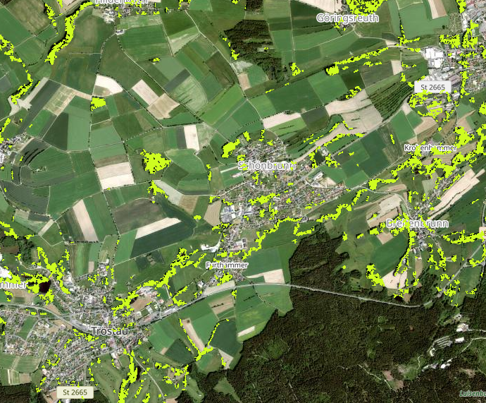
Display of a single band from a VRT file:
# Import libraries
from IPython.display import display
from vois.geo import Map
from geolayer import rasterlayer

# Create a single rasterlayer istance to display the first band of a VRT file
ly = rasterlayer.single('.../SWF2018/VER1-0/Data/VRT/SWF_2018_005m_03035_V1_0.vrt',
                        band=1, epsg=3035, nodata=0.0)

# Display all pixels having value 1 with a pale green color
# (see colorizer() and color() for a complete description)
ly.color(value=1.0, color="#cefc20", mode="exact")

# Create a Map
m = Map.Map(zoom=14, basemapindex=1)

# Add the layer to the map
m.addLayer(ly)

# Set the identify operation
m.onclick = ly.onclick

# Display the map
display(m)
- classmethod rgb(filepath, bandR=1, bandG=2, bandB=3, epsg=None, nodata=None, scalemin=None, scalemax=None, scaling='near', opacity=1.0)
RGB composition of three bands of a raster dataset.
- Parameters:
filepath (str) – File path of the raster to display.
bandR (int, optional) – Band number (from 1 to n) to display in the Red channel (default is 1).
bandG (int, optional) – Band number (from 1 to n) to display in the Green channel (default is 2).
bandB (int, optional) – Band number (from 1 to n) to display in the Blue channel (default is 3).
epsg (int, optional) – EPSG code of the coordinate system to use (default is 4326, the geographical coordinates).
nodata (float, optional) – Value to be cosidered as absence of data (default is 999999.0).
scaling (str, optional) – Scaling mode (one of ‘near’, ‘fast’, ‘bilinear’, ‘bicubic’, ‘spline16’, ‘spline36’, ‘hanning’, ‘hamming’, ‘hermite’, ‘kaiser’, ‘quadric’, ‘catrom’, ‘gaussian’, ‘bessel’, ‘mitchell’, ‘sinc’, ‘lanczos’, ‘blackman’). Default is ‘near’.
scalemin (float or list of 3 floats, optional) – Minimum scaling value to convert from raster values to the interval [0,255] (default is None)
scalemax (float or list of 3 floats, optional) – Maximum scaling value to convert from raster values to the interval [0,255] (default is None)
opacity (float, optional) – Opacity value (from 0.0 to 1.0) to display the RGB composition with partial transparency (default is 1.0, fully opaque)
Example
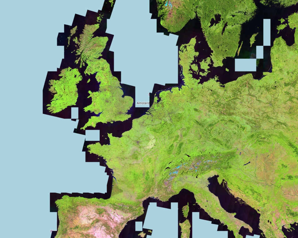
Display of a RGB composition from a VRT file:
# Import libraries
from IPython.display import display
from vois.geo import Map
from geolayer import rasterlayer

# Create a RGB composition istance to display bands 3,2,1 of a VRT file
ly = rasterlayer.rgb('.../GLOBAL/UMD/GFC/VER1-7/Data/VRT/last/Hansen_GFC-2019-v1.7_last.vrt',
                     nodata=0.0,
                     bandR=3,
                     bandG=2,
                     bandB=1,
                     scalemin=[0.0, 0.0, 0.0],
                     scalemax=[120.0, 100.0, 105.0],
                     scaling='bilinear')

# Create a Map
m = Map.Map()

# Add the layer to the map
m.addLayer(ly)

# Set the identify operation
m.onclick = ly.onclick

# Display the map
display(m)
- classmethod hillshade(filepath, band=1, epsg=None, nodata=None, scaling='near', opacity=1.0, azimut=315.0, elevation=45.0, zfactor=1.0)
Digital Elevation Model visualization in grayscale hillshading mode.
- Parameters:
filepath (str) – File path of the input DEM raster file.
band (int, optional) – Band number (from 1 to n) to display (default is 1).
epsg (int, optional) – EPSG code of the coordinate system to use. If None, the epsg of the input DEM file is used (default is None).
nodata (float, optional) – Value to be cosidered as absence of data. If None, the nodata value of the input DEM file is used (default is None).
scaling (str, optional) – Scaling mode (one of ‘near’, ‘fast’, ‘bilinear’, ‘bicubic’, ‘spline16’, ‘spline36’, ‘hanning’, ‘hamming’, ‘hermite’, ‘kaiser’, ‘quadric’, ‘catrom’, ‘gaussian’, ‘bessel’, ‘mitchell’, ‘sinc’, ‘lanczos’, ‘blackman’). Default is ‘near’.
opacity (float, optional) – Opacity value (from 0.0 to 1.0) to display the RGB composition with partial transparency (default is 1.0, fully opaque)
azimut (float, optional) – Horizontal angle in degrees of the sun position calculated from North in clockwise direction [0,360] (default is 315.0, northwest direction which maximizes the relief effect)
elevation (float, optional) – Elevation of the sun position over the horizon in degrees [0,90] (default is 45.0)
zfactor (float, optional) – Multiplying factor to increase or decrease the heights (default is 1.0)
Example
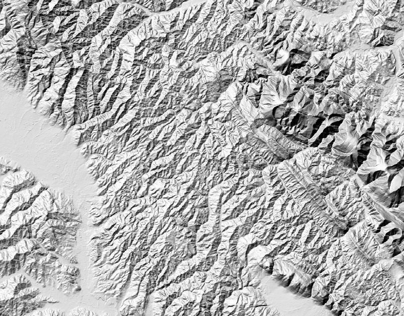
Display of a DEM in grayscale hillshading mode:
# Import libraries
from IPython.display import display
from vois.geo import Map
from geolayer import rasterlayer

demfile = '.../GLOBAL/COP-DEM/GLO-30-DGED/VER1-0/Data/VRT/Copernicus_DSM_10.vrt'

ly = rasterlayer.hillshade(demfile, band=1, elevation=60, zfactor=4, opacity=1)

# Create a Map
m = Map.Map()

# Add the layer to the map
m.addLayer(ly)

# Display the map
display(m)
- classmethod hillshadeColors(filepath, band=1, epsg=None, nodata=None, scaling='near', opacity=1.0, azimut=315.0, elevation=45.0, zfactor=1.0, scalemin=0.0, scalemax=1500.0, colorlist=['#ffffaa', '#27a827', '#0b8040', '#ffff00', '#ffba03', '#9e1e02', '#6e280a', '#8a5e42', '#ffffff'])
Digital Elevation Model visualization in coloured hillshading mode.
- Parameters:
filepath (str) – File path of the input DEM raster file.
band (int, optional) – Band number (from 1 to n) to display (default is 1).
epsg (int, optional) – EPSG code of the coordinate system to use. If None, the epsg of the input DEM file is used (default is None).
nodata (float, optional) – Value to be cosidered as absence of data. If None, the nodata value of the input DEM file is used (default is None).
scaling (str, optional) – Scaling mode (one of ‘near’, ‘fast’, ‘bilinear’, ‘bicubic’, ‘spline16’, ‘spline36’, ‘hanning’, ‘hamming’, ‘hermite’, ‘kaiser’, ‘quadric’, ‘catrom’, ‘gaussian’, ‘bessel’, ‘mitchell’, ‘sinc’, ‘lanczos’, ‘blackman’). Default is ‘near’.
opacity (float, optional) – Opacity value (from 0.0 to 1.0) to display the RGB composition with partial transparency (default is 1.0, fully opaque)
azimut (float, optional) – Horizontal angle in degrees of the sun position calculated from North in clockwise direction [0,360] (default is 315.0, northwest direction which maximizes the relief effect)
elevation (float, optional) – Elevation of the sun position over the horizon in degrees [0,90] (default is 45.0)
zfactor (float, optional) – Multiplying factor to increase or decrease the heights (default is 1.0)
scalemin (float, optional) – Elevation assigned to the first color of the colorlist (default is 0.0). Colors are linearly assigned to the elevation range [scalemin,scalemax].
scalemax (float, optional) – Elevation assigned to the last color of the colorlist (default is 0.0). Colors are linearly assigned to the elevation range [scalemin,scalemax].
colorlist (list of str in '#rrggbb' format, optional) – Color palette to use for elevation values. Default is [‘#ffffaa’, ‘#27a827’, ‘#0b8040’, ‘#ffff00’, ‘#ffba03’, ‘#9e1e02’, ‘#6e280a’, ‘#8a5e42’, ‘#ffffff’]
Example
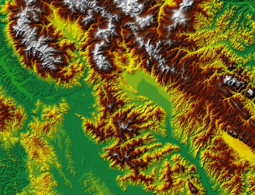
Display of a DEM in coloured hillshading mode:
# Import libraries
from IPython.display import display
from vois.geo import Map
from geolayer import rasterlayer

demfile = '.../GLOBAL/COP-DEM/GLO-30-DGED/VER1-0/Data/VRT/Copernicus_DSM_10.vrt'

ly = rasterlayer.hillshadeColors(demfile, band=1,
                                 elevation=60, zfactor=4, opacity=1,
                                 scalemax=1000)

# Create a Map
m = Map.Map()

# Add the layer to the map
m.addLayer(ly)

# Display the map
display(m)
- classmethod sentinel2single(stacitem, band='B04', scalemin=None, scalemax=None, colorlist=['#000000', '#ffffff'], scaling='near', opacity=1.0)
Display a single band of a Sentinel-2 L2A product. The input product can be selected by passing its Product ID string (i.e: ‘S2A_MSIL2A_20230910T100601_N0509_R022_T32TQP_20230910T161500’) or the dict returned by a call to the
sentinel2item()method.The assignment of a list of colors to the pixel values is done by linearly mapping the range of pixel values [scalemin, scalemax] to the color palette. If None is passed as parameters scalemin and scalemax, the statistics of the input band are used to calculate the scaling parameters as [avg - 2*stddev, avg + 2*stddev].
- Parameters:
stacitem (str or dict, optional) – Product ID string of the Sentinel-2 L2A product or the dict returned by a call to the
sentinel2item()method containing the product metadata.band (str, optional) – Band name of the band to display (default is ‘B04’).
scalemin (float, optional) – Minimum pixel value to define the range of pixel values assigned to the list or colors. The default value is None.
scalemin – Maximum pixel value to define the range of pixel values assigned to the list or colors. The default value is None.
colorlist (list of str, optional) – List of strings defining the colors. Common names of colors can be used (i.e ‘red’) or their exadecimal RGB representation ‘#rrggbb’. The default colorlist is [‘#000000’,’#ffffff’] which defines a shades of gray color ramp.
scaling (str, optional) – Scaling mode (one of ‘near’, ‘fast’, ‘bilinear’, ‘bicubic’, ‘spline16’, ‘spline36’, ‘hanning’, ‘hamming’, ‘hermite’, ‘kaiser’, ‘quadric’, ‘catrom’, ‘gaussian’, ‘bessel’, ‘mitchell’, ‘sinc’, ‘lanczos’, ‘blackman’). Default is ‘near’.
opacity (float, optional) – Opacity value (from 0.0 to 1.0) to display raster with partial transparency (default is 1.0, fully opaque).
Example
Display of band B04 of a Sentinel-2 L2A product (using one of the Plotly continuous color scales):
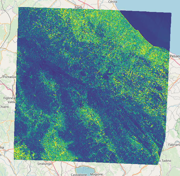
# Import libraries
from IPython.display import display
from vois.geo import Map
from geolayer import rasterlayer
import plotly.express as px

# Create a rasterlayer istance to display a single Sentinel-2 band
ly = rasterlayer.sentinel2single('S2A_MSIL2A_20230910T100601_N0509_R022_T32TQP_20230910T161500',
                                 band='B04',
                                 scaling='near',
                                 scalemin=800,
                                 scalemax=2800,
                                 colorlist=px.colors.sequential.Viridis)

# Create a Map
m = Map.Map(center=[43.696, 12.1179], zoom=9)

# Add the layer to the map
m.addLayer(ly)

# Set the identify operation
m.onclick = ly.onclick

# Display the map
display(m)
- classmethod sentinel2rgb(stacitem, bandR='B04', bandG='B03', bandB='B02', scalemin=None, scalemax=None, scaling='near', opacity=1.0)
Display an RGB three bands composition of a Sentinel-2 L2A product. The input product can be selected by passing its Product ID string (i.e: ‘S2A_MSIL2A_20230910T100601_N0509_R022_T32TQP_20230910T161500’) or the dict returned by a call to the
sentinel2item()method.The assignment of colors to the pixel values is done by linearly mapping the range of pixel values [scalemin, scalemax] to the [0, 255] interval. If None is passed as parameters scalemin and scalemax, the statistics of the input bands are used to calculate the scaling parameters as [avg - 2*stddev, avg + 2*stddev] for each of the three input bands.
- Parameters:
stacitem (str or dict, optional) – Product ID string of the Sentinel-2 L2A product or the dict returned by a call to the
sentinel2item()method containing the product metadata.bandR (str, optional) – Band name of the band to display in the Red channel (default is ‘B04’).
bandG (str, optional) – Band name of the band to display in the Green channel (default is ‘B03’).
bandB (str, optional) – Band name of the band to display in the Blue channel (default is ‘B02’).
scalemin (float or list of 3 floats, optional) – Minimum pixel value to define the range of pixel values mapped to the [0, 255] visualization range. If a single float values is passes, the same scalemin value is used for all the three input bands. As an alternative a list of three floats can be passed to specify distinct values for each of the bands. The default value is None, allowing for automatic calculation of input range from the three bands statistics.
scalemin – Maximum pixel value to define the range of pixel values mapped to the [0, 255] visualization range. If a single float values is passes, the same scalemax value is used for all the three input bands. As an alternative a list of three floats can be passed to specify distinct values for each of the bands. The default value is None, allowing for automatic calculation of input range from the three bands statistics.
scaling (str, optional) – Scaling mode (one of ‘near’, ‘fast’, ‘bilinear’, ‘bicubic’, ‘spline16’, ‘spline36’, ‘hanning’, ‘hamming’, ‘hermite’, ‘kaiser’, ‘quadric’, ‘catrom’, ‘gaussian’, ‘bessel’, ‘mitchell’, ‘sinc’, ‘lanczos’, ‘blackman’). Default is ‘near’.
opacity (float, optional) – Opacity value (from 0.0 to 1.0) to display raster with partial transparency (default is 1.0, fully opaque).
Example
Display of a True Color RGB composition (B04/B03/B02) of a Sentinel-2 L2A product (using the bands statistics to calculate the optimal scaling ranges):
# Import libraries
from IPython.display import display
from vois.geo import Map
from geolayer import rasterlayer

# Create a rasterlayer istance to display a RGB composition of a Sentinel-2 L2A product
ly = rasterlayer.sentinel2rgb('S2A_MSIL2A_20230910T100601_N0509_R022_T32TQP_20230910T161500')

# Create a Map
m = Map.Map(center=[43.696, 12.1179], zoom=9)

# Add the layer to the map
m.addLayer(ly)

# Set the identify operation
m.onclick = ly.onclick

# Display the map
display(m)

- classmethod sentinel2index(stacitem, band1='B08', band2='B04', scalemin=0, scalemax=0.75, colorlist=['#784519', '#ffb24a', '#ffeda6', '#ade85e', '#87b540', '#039c00', '#016400', '#015000'], scaling='near', opacity=1.0)
Display an index calculated from 2 bands (b1 - b2)/(b1 + b2) of a Sentinel-2 L2A product. The input product can be selected by passing its Product ID string (i.e: ‘S2A_MSIL2A_20230910T100601_N0509_R022_T32TQP_20230910T161500’) or the dict returned by a call to the
sentinel2item()method. The index calculation returns pixel values in the range [-1, 1].The assignment of colors to the pixel values is done by linearly mapping the range of pixel values [scalemin, scalemax] to the color ramp.
- Parameters:
stacitem (str or dict, optional) – Product ID string of the Sentinel-2 L2A product or the dict returned by a call to the
sentinel2item()method containing the product metadata.band1 (str, optional) – Band name of the first band to use for the index calculation (default is ‘B08’).
band2 (str, optional) – Band name of the second band to use for the index calculation (default is ‘B04’).
scalemin (float, optional) – Minimum pixel value to define the range of pixel values mapped to the colorlist colors. Default is 0.0.
scalemin – Maximum pixel value to define the range of pixel values mapped to the colorlist colors. Default is 0.75.
colorlist (list of str, optional) – List of strings defining the colors. Common names of colors can be used (i.e ‘red’) or their exadecimal RGB representation ‘#rrggbb’. The default colorlist is a brown-to-green color ramp.
scaling (str, optional) – Scaling mode (one of ‘near’, ‘fast’, ‘bilinear’, ‘bicubic’, ‘spline16’, ‘spline36’, ‘hanning’, ‘hamming’, ‘hermite’, ‘kaiser’, ‘quadric’, ‘catrom’, ‘gaussian’, ‘bessel’, ‘mitchell’, ‘sinc’, ‘lanczos’, ‘blackman’). Default is ‘near’.
opacity (float, optional) – Opacity value (from 0.0 to 1.0) to display raster with partial transparency (default is 1.0, fully opaque).
Example
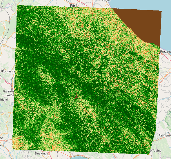
Display of an NDVI index (B08 - B04)/(B08 + B04) of a Sentinel-2 L2A product:
# Import libraries
from IPython.display import display
from vois.geo import Map
from geolayer import rasterlayer

# Create a rasterlayer istance to display the NDVI index on a Sentinel-2 product
ly = rasterlayer.sentinel2index('S2A_MSIL2A_20230910T100601_N0509_R022_T32TQP_20230910T161500',
                                band1='B08',
                                band2='B04',
                                scaling='near',
                                scalemin=0.0,
                                scalemax=0.6)

# Create a Map
m = Map.Map(center=[43.696, 12.1179], zoom=9)

# Add the layer to the map
m.addLayer(ly)

# Set the identify operation
m.onclick = ly.onclick

# Display the map
display(m)
- static sentinel2item(S2_L2A_Product_ID)
Given in input a string containing the Product ID of a Sentinel-2 L2A producs (i.e: ‘S2A_MSIL2A_20230910T100601_N0509_R022_T32TQP_20230910T161500’), this static method of the rasterlayer class returns the full stacitem of the product (a dict containing all the metadata information of the product).
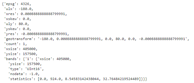
- static info(filepath)
Returns a dict containing info on a raster file.
- Parameters:
filepath (str) – Full path of the raster file.
Example
Request info on a VRT raster file:
# Import libraries
from IPython.display import display
from geolayer import rasterlayer

info = rasterlayer.info('/eos/jeodpp/data/base/Energy/EUROPE/ESA/Biomass_cci/VER3-0/Data/VRT/2018/2018_ESACCI_BIOMASS-L4-AGB.vrt')
display(info)
- print()
Prints a textual description of the class instance.
- symbolizer(scaling='near', opacity=1.0, composition='')
Initialize the raster rendering by providing settings for single-band display. The geolayer library uses Mapnik to render a raster dataset. See the see Raster Symbolizer description for info.
After a rasterlayer instance is created, this method must be called only if a non-default setting is needed. In other words, if the created rasterlayer instance is going to be displayed using near-neighbour interpolation and fully opaque, the call to simbolizer() method can be avoided.
- Parameters:
scaling (str, optional) – Scaling mode (one of ‘near’, ‘fast’, ‘bilinear’, ‘bicubic’, ‘spline16’, ‘spline36’, ‘hanning’, ‘hamming’, ‘hermite’, ‘kaiser’, ‘quadric’, ‘catrom’, ‘gaussian’, ‘bessel’, ‘mitchell’, ‘sinc’, ‘lanczos’, ‘blackman’). Default is ‘near’.
opacity (float, optional) – Opacity value (from 0.0 to 1.0) to display raster with partial transparency (default is 1.0, fully opaque).
composition (str, optional) – Compositing/Merging effects with image below raster level. Possible values are: grain_merge, grain_merge2, multiply, multiply2, divide, divide2, screen, hard_light. Default is ‘’.
- colorizer(default_mode='linear', default_color='transparent', epsilon=1.5e-07)
Create a colorizer descriptor to define how the values of a single-band raster are transformed into colors. See the Raster Colorizer help page for more details.
The colorizer works in the following way:
It has an ordered list of stops that describe how to translate an input value to an output color.
A stop has a value, which marks the stop as being applied to input values from its value, up until the next stops value.
A stop has a mode, which says how the input value will be converted to a colour.
A stop has a color
The colorizer also has default color, which input values will be converted to if they don’t match any stops.
The colorizer also has a default mode, which can be inherited by the stops.
The colorizer also has an epsilon value, which is used in the exact mode.
Modes
The available modes are inherit, discrete, linear, and exact.
inherit is only valid for stops, and not the default colorizer mode. It means that the stop will inherit the mode of the containing colorizer.
discrete causes all input values from the stops value, up until the next stops value (or forever if this is the last stop) to be translated to the stops color.
linear causes all input values from the stops value, up until the next stops value to be translated to a color which is linearly interpolated between the two stops colors. If there is no next stop, then the discrete mode will be used.
exact causes an input value which matches the stops value to be translated to the stops color. The colorizers epsilon value can be used to make the match a bit fuzzy (in the ‘greater than’ direction).
The colorizer method sets the initial parameters of the Colorizer. To add one or more stops to the colorizer the following methods can be called:
After a rasterlayer instance is created, this method must be called only if a non-default setting is needed. In other words, if the created rasterlayer instance is going to be displayed using the “linear” mode and the “transparent” default color, the call to the colorizer() method can be avoided.
- Parameters:
default_mode (str, optional) – Default colorizer mode that can be inherited by all subsequent stops in case the inherit mode is selected. Default is ‘linear’.
default_color (str, optional) – Starting color of the first step of the colorizer. Default is ‘transparent’.
epsilon (float, optional) – Error threshold used in the exact mode to decide if a pixel value matches a stop value. Default is 1.5e-07.
Examples
To visualize a raster mask band by assigning a color to the “valid” pixels:
ly = rasterlayer.single('...', band=1, epsg=3035, nodata=0.0)
ly.color(value=1.0, color="#cefc20", mode="exact")
To visualize a raster band by assigning a palette of colors to a range of pixel values:
ly = rasterlayer.single('...', band=1, epsg=3035, nodata=0.0)
ly.colorlist(0.0, 100.0, ['#ff0000', '#0000ff'])
To visualize a raster band by using a mapping of pixel values to specific colors:
ly = rasterlayer.single('...', band=1, epsg=3035, nodata=0.0)
ly.colormap({1.0: 'red',
             2.0: '#ffff00',
             3.0: '#00ffff',
             4.0: '#0000ff',
             5.0: '#aaffaa'})
- color(value, color='red', mode='linear')
Add a colorizer stop. Read the description of the method
colorizer()or open the Raster Colorizer help page for more details.- Parameters:
value (float) – Numerical value of the raster pixel at which the stop begins to be applied.
color (str, optional) – Color assigned to the stop. If not specified, the colorizers default_color will be used. A name of color or its exadecimal representation ‘#rrggbb’ can be used. Default is ‘red’.
mode (str, optional) – Stop mode: defines how the assignment of colors is implemented. Possible modes are ‘discrete’, ‘exact’ or ‘linear’ (default).
- colorlist(scalemin, scalemax, colorlist)
Add a series of colorizer stops, one for each item of a list of colors, so that the pixel values inside a range [scalemin, scalemax] are linearly assigned to the colors of the list. Read the description of the method
colorizer()for an example.- Parameters:
scalemin (float) – Minimum pixel value to define the range of pixel values assigned to the list or colors.
scalemin – Maximum pixel value to define the range of pixel values assigned to the list or colors.
colorlist (list of str) – List of strings defining the colors. Common names of colors can be used (i.e ‘red’) or their exadecimal RGB representation ‘#rrggbb’.
- colormap(values2colors, mode='linear')
Add a series of colorizer stops from a dictionary that maps some pixel values to specific colors. Read the description of the method
colorizer()for an example.
- identify(lon, lat, zoom)
Given in input a geographic coordinate and a zoom level, returns a scalar float/int/string or a list of scalars containing info on the pixel under the (lat,lon) position.
- Parameters:
- Returns:
res – A scalar float/int/string or a list of scalars
- Return type:
float/int/string or list of float/int/string
- property identify_dict
Get/Set the dictionary to be used in the identify operation (click on a pixel) to convert a numerical pixel value into a string description. It can be useful to display class names instead of numerical values when querying categorical raster bands (datasets where each integer value represents a class or category)
- Returns:
d – Dictionary that assigns a string to each pixel value.
- Return type:
Example
Programmatically change the identify dictionary:
vlayer.identify_dict = {1: 'wheat', 2: 'maize'}
print(vlayer.identify_dict)
- property identify_integer
Get/Set the flag that requests the identify operation (click on a pixel) to return an integer value.
- Returns:
flag – True if the identify operation must return an integer value.
- Return type:
Example
Programmatically change the identify integer flag:
vlayer.identify_integer = True
print(vlayer.identify_integer)
- property identify_digits
Get/Set the flag number of digits to use for the display of floating point values in an identify operation (click on a pixel).
- Returns:
n – Number of decimal digits to use for the display of floating point pixel values.
- Return type:
Example
Programmatically change the identify_digits value:
vlayer.identify_digits = 2
print(vlayer.identify_digits)
- property identify_label
Get/Set the string to use in the display of an identify operation (click on a pixel).
- Returns:
label – Label to prepend to the pixel values displayed in an identify operation.
- Return type:
Example
Programmatically change the identify_label value:
vlayer.identify_label = 'Intensity value'
print(vlayer.identify_label)
- tileLayer(max_zoom=22)
Creates an ipyleaflet.TileLayer object from an instance of rasterlayer, to be added to a Map for display.
- Returns:
tlayer – Instance of ipyleaflet.TileLayer to be added to a Map
- Return type:
ipyleaflet.TileLayer
Example
Create an ipyleaflet.TileLayer instance:
# Import libraries
from IPython.display import display
import ipyleaflet
from geolayer import rasterlayer

# Create a rasterlayer instance
rlayer = rasterlayer.single(...)

# Create an ipyleaflet Map
m = ipyleaflet.Map()

# Add the layer to the map
m.add(rlayer.tileLayer())

# Display the map
display(m)
vectorlayer
Tip
The chapter Display vector datasets contains a guide on how symbology can be defined for vector datasets display. To visually edit symbols for vector datasets display, please use the Symbol Editor described in chapter Create symbols for vector datasets.
Display of vector datasets (shapefiles, geopackage, POSTGIS queries and WKT strings) on a ipyleaflet Map
- class vectorlayer.vectorlayer(filepath='', layer='', epsg=4326, proj='', identify_fields=[])
Vector datasets visualization. Class to display vector file datasets (shapefiles, geopackage, etc.), WKT strings (see: Well Known Text format) and POSTGIS geospatial tables and queries.
An instance of this class can be created using one of these class methods:
To apply symbology to a vectorlayer class, these methods can be used:
A parametric symbol can be defined using tags like FILL-COLOR, STROKE-WIDTH, etc. that can be substituted with real values using the static method
symbolChange().See the chapter Display vector datasets for a guide on how symbols are defined and the chapter Create symbols for vector datasets for help on the visual Symbol Editor.
- classmethod file(filepath, layer=None, epsg=None, proj='')
Display of a file-based vector dataset on an ipyleaflet Map.
- Parameters:
filepath (str) – File path of the vector dataset to display (shapefile, geopackage, etc.).
layer (str, optional) – Name of the layer to display (for a shapefile it can be None). Default is None.
epsg (int, optional) – EPSG code of the coordinate system to use (default is None meaning that the geolayer library will try to understand the EPSG code itself).
proj (str, optional) – Proj4 string of the coordinate system to use (default is the empty string). If a non-empty string is passed, the proj parameter has prevalence over the epsg code.
Example
Display of a shapefile:
# Import libraries
from IPython.display import display
from vois.geo import Map
from geolayer import vectorlayer

# Create a vectorlayer instance from a file dataset (shapefile)
vlayer = vectorlayer.file('.../NUTS_RG_03M_2021_4326_0.shp', epsg=4326)

# Define a parametric symbol ('FILL-COLOR' to be substituted with the actual color)
symbol = [
            [
               ["PolygonSymbolizer", "fill", 'FILL-COLOR'],
               ["PolygonSymbolizer", "fill-opacity", 0.8],
               ["LineSymbolizer", "stroke", "#000000"],
               ["LineSymbolizer", "stroke-width", 1.0]
            ]
]

# Remove default symbology
vlayer.symbologyClear()

# Assign a red symbol to all features
vlayer.symbologyAdd(symbol=vectorlayer.symbolChange(symbol, fillColor='red'))

# Assign a green symbol to a subset of the features
vlayer.symbologyAdd(rule="[CNTR_CODE] = 'IT'",
                    symbol=vectorlayer.symbolChange(symbol, fillColor='#00aa00'))

# Create a Map
m = Map.Map()

# Add the layer to the map
m.addLayer(vlayer)

# Set the identify operation
m.onclick = vlayer.onclick

# Display the map
display(m)
- classmethod wkt(wktlist, properties=[])
Display of one or more WKT (Well-Known-Text) strings as geospatial vector features over an ipyleaflet Map.
- Parameters:
List of strings in WKT format containing the geometry of features to display (see: Well Known Text format).
properties (list of dict, optional) – List of dict containing attributes of the features (default is []).
Example
Display of a WKT string:
# Import libraries
from IPython.display import display
from vois.geo import Map
from geolayer import vectorlayer

# Create a vectorlayer instance from a WKT string
vlayer = vectorlayer.wkt(['POLYGON ((20 40, 0 45, 10 52, 30 52, 20 40))'],
                         [{"ndx": 22, "value": 12.8798, "units": "abcd"}])

# Define a symbol
symbol = [
            [
               ["PolygonSymbolizer", "fill", '#0088ff'],
               ["PolygonSymbolizer", "fill-opacity", 0.8],
               ["LineSymbolizer", "stroke", "#000000"],
               ["LineSymbolizer", "stroke-width", 4.0]
            ]
]

# Remove default symbology
vlayer.symbologyClear()

# Assign a symbol to a subset of the features
vlayer.symbologyAdd(rule="[units] = 'abcd'", symbol=symbol)

# Create a Map
m = Map.Map()

# Add the layer to the map
m.addLayer(vlayer)

# Set the identify operation
m.onclick = vlayer.onclick

# Display the map
display(m)
- classmethod postgis(host, port, dbname, user, password, query, epsg=4326, proj='', geomtype='Polygon', geometry_field='', geometry_table='', extents='')
Display of a POSTGIS geospatial query over an ipyleaflet Map.
- Parameters:
host (str) – Address for the POSTGIS server. You can use an IP address or the hostname of the machine on which database server is running.
port (int) – Port on which you have configured your POSTGIS instance while installing or initializing. The default port is 5432.
dbname (str) – The name of the database with which you want to connect. The default name of the database is the same as that of the user.
user (str) – User name to be used for the connection to the POSTGIS database.
password (str) – Password for the user name.
query (str) – Query in SQL format to extract information from the DB. It should include a geoemtry field.
epsg (int, optional) – EPSG code of the coordinate system to use (default is 4326, the geographical coordinates).
proj (str, optional) – Proj4 string of the coordinate system to use (default is the empty string). If a non-empty string is passed, the proj parameter has prevalence over the epsg code.
geomtype (str, optional) – Geometry type of the features returned by the query. In can be ‘Polygon’, ‘LineString’ or ‘Point’. Default is ‘Polygon’.
geometry_field (str, optional) – Name of the geometry field, in case you have more than one in a single table. This field will be deduced from the query in most cases, but may need to be manually specified in some cases. Default is ‘’.
geometry_table (str, optional) – Name of table geometry is retrieved from. Auto detected when not given, but this may fail for complex queries. Default is ‘’.
extents (str, optional) –
Maximum extent of the geometries in the format “xmin ymin, xmax ymax”; if omitted, the extents will be determined by querying the metadata for the table.
Important!: always pass a valid extents string, since this will make the display much faster in most cases.
Example
Display of a POSTGIS query:
# Import libraries
from IPython.display import display
from vois.geo import Map
from geolayer import vectorlayer

# Create a vectorlayer instance for a POSTGIS query
vlayer = vectorlayer.postgis(
            host="XXXXXX",
            port=5432,
            dbname="XXXXXX",
            user="XXXXXX",
            password="XXXXXX",
            query="SELECT geom FROM mytable",
            epsg=3035,
            geomtype="Polygon",
            extents="4200207.5 3496795.9,4649995.8 3848272.9")

# Define a symbol
symbol = [
            [
               ["PolygonSymbolizer", "fill", '#ff0000'],
               ["PolygonSymbolizer", "fill-opacity", 0.3],
               ["LineSymbolizer", "stroke", "#000000"],
               ["LineSymbolizer", "stroke-width", 1.0]
            ]
]

# Remove default symbology
vlayer.symbologyClear()

# Assign the symbol to all the features of the query
vlayer.symbologyAdd(symbol=symbol)

# Create a Map
m = Map.Map()

# Add the layer to the map
m.addLayer(vlayer)

# Set the identify operation
m.onclick = vlayer.onclick
vlayer.identify_fields = ['FID', 'GEOMETRY']

# Display the map
display(m)
- static layers(filepath)
Returns the list of layers of a file-based vector dataset (shapefile, geopackage, sqlite, etc.).
- Parameters:
filepath (str) – Full path of the file-based dataset (shapefile, geopackage, sqlite, etc.).
- static layer(filepath, layer=None)
Returns a dictionary containing info on a layer of a file-based vector dataset (extent, feature type, feature count, epsg, etc.).
- fields()
Returns a dictionary containing info on the fields of a file-based vector dataset. Works only for a filebased or a wkt instance.
- field(field)
Returns a dictionary containing info on a field of a file-based vector dataset. Works only for a filebased or a wkt instance.
- Parameters:
field (str) – Name of the field to query.
- values(field)
Returns the list of all values of a field of a layer. Works only for a filebased or a wkt instance.
- Parameters:
field (str) – Name of the field to query.
- distinct(field)
Returns a dictionary of all the distinct values of a field of a layer of a dataset with their number of occurrencies. Works only for a filebased or a wkt instance.
- Parameters:
field (str) – Name of the field to query.
- stats(field)
Returns a dictionary containing statistical information on a numeric field of a layer of a dataset. Works only for a filebased or a wkt instance.
- Parameters:
field (str) – Name of the field to query.
- symbologyClear(maxstyle=0)
Remove all the default symbology for a vectorlayer instance and all the symbols eventually added. By default a vectorlayer instance has a default symbology (for instance a pale yellow for polygons) so that it can be displayed even if no symbology is added using the
symbologyAdd(). By calling symbologyClean method, all these default display settings are removed.- Parameters:
maxstyle (int, optional) – A symbol in geolayer can have a maximum of 10 layers (corresponding to the number of lists inside its definition. The first list will be mapped to style0, the second to style1, etc., up to style9). This parameter can be used to clear only the first style (style0) if 0 is passed (default), or up to all the styles if 10 is passed. If the symbols you use are only made of a single layer, call this function without specifying the maxstyle parameter, since the default value of 0 is sufficient to clean the symbology.
- symbologyAdd(rule='all', symbol=[])
Add a new symbology rule.
- Parameters:
rule (str, optional) – Filter to define the feature that will be rendered with the symbol. Passing ‘all’ applies the symbol to all the features, while a filter like “[attrib] = ‘value’” makes the symbol applied only to a subset of the features. See Mapnik Filter Syntax for help in writing the filter. Default is ‘all’.
symbol (list of lists, optional) – Symbol to be used for the rendering of the features. See the chapter Display vector datasets for a guide on how symbols are defined and the chapter Create symbols for vector datasets for help on the visual Symbol Editor.
- legendSingle(symbol=[], description='')
Create a legend that uses a single symbol for all the features.
- Parameters:
symbol (list of lists, optional) – Symbol to be used for the rendering of the features. See the chapter Display vector datasets for a guide on how symbols are defined and the chapter Create symbols for vector datasets for help on the visual Symbol Editor.
description (str, optional) – Description of the unique item of the legend (default is ‘’).
- Returns:
legend – A legend is a list of dictionaries, one for each item. Each dict contains the keys: description, rule and symbol
- Return type:
list of dicts
- legendCategories(fieldname, colorlist, symbol=[], interpolate=True, distinctValues=None)
Create a legend containing one item for each distinct value of a field. In case of file-based datasets (shapefiles, geopackage, aqlite, etc.) or wkt datasets, given a fieldname, the distinct values of this field are retrieved by the method legendCategories itself. On the contrary, for a postgis vectorlayer instance, the distinctValues parameter must be passed containing the list of all the unique values of the field (it is responsibility of the user to retrieve this list using a call to the underlying DB).
- Parameters:
fieldname (str) – Name of the field whose distinct values must be used.
colorlist (list of str) – List of colors to be used for the creation of the legend. See Plotly sequential color scales and Plotly qualitative color sequences for possible color lists.
symbol (list of lists, optional) – Symbol to be used for the rendering of the features. See the chapter Display vector datasets for a guide on how symbols are defined and the chapter Create symbols for vector datasets for help on the visual Symbol Editor.
interpolate (bool, optional) – If True, the colors assigned to the items of the legend are calculated by using linear interpolation on the list of colors (thus potentially generating also intermediate colors). If False, only the colors in the list are used. In this case, if the number of distinct values is greated than the number of colors in the list, some legend items will have repeated colors.
distinctValues (list, optional) – Custom list of distinct values to use for the creation of the legend. Default is None, meaning that, for filebased and wkt vectorlayer instances, the list of distinct values is autonomously calculated. This parameter must be mandatory passed when the vectorlayer instance is a postgis dataset.
- Returns:
legend – A legend is a list of dictionaries, one for each item. Each dict contains the keys: description, rule and symbol
- Return type:
list of dicts
Example
Create a categories legend on a field of a shapefile:
# Import libraries
from IPython.display import display
from geolayer import vectorlayer
import plotly.express as px

# Create a vectorlayer instance from a file dataset (shapefile)
vlayer = vectorlayer.file('.../NUTS_RG_03M_2021_4326_0.shp')

# Define a parametrical symbol
symbol = [
            [
               ["PolygonSymbolizer", "fill", 'FILL-COLOR'],
               ["PolygonSymbolizer", "fill-opacity", 0.8],
               ["LineSymbolizer", "stroke", "#000000"],
               ["LineSymbolizer", "stroke-width", 1.0]
            ]
]

# Create a legend on the distinct values of the CNTR_CODE field
legend = vlayer.legendCategories('CNTR_CODE',
                                 px.colors.qualitative.Dark24,
                                 symbol=symbol,
                                 interpolate=False)
- legendGraduated(fieldname, colorlist, symbol=[], allValues=None, classifier_name='Quantiles', classifier_param1=5, classifier_param2=None, interpolate=True, markersize_min=1.0, markersize_max=1.0, digits=2)
Create a legend on the graduated values of a numerical field. In case of file-based datasets (shapefiles, geopackage, aqlite, etc.) or wkt datasets, given a fieldname, the values of this field are retrieved by the method legendGraduated itself. On the contrary, for a postgis vectorlayer instance, the allValues parameter must be passed containing the list of all the values of the field (it is responsibility of the user to retrieve this list using a call to the underlying DB).
See mapclassify help for additional guidance.
Each of the different classification methods takes one or more input parameters:
‘EqualInterval’: classifier_param1 = the number of classes required
‘BoxPlot’: None
‘NaturalBreaks’: classifier_param1 = the number of classes required
‘FisherJenksSampled’: classifier_param1 = the number of classes required, classifier_param1 = the percentage of values that should form the sample (standard value is 0.1)
‘StdMean’: classifier_param1 = a list containing the multiples of the standard deviation to add/subtract from the sample mean to define the bins (example [-2, -1, 1, 2]
‘JenksCaspallForced’: classifier_param1 = the number of classes required
‘HeadTailBreaks’: None
‘Quantiles’: classifier_param1 = the number of classes required
- Parameters:
fieldname (str) – Name of the field whose values must be used.
colorlist (list of str) – List of colors to be used for the creation of the legend.
symbol (list of lists, optional) – Symbol to be used for the rendering of the features. See the chapter Display vector datasets for a guide on how symbols are defined and the chapter Create symbols for vector datasets for help on the visual Symbol Editor.
allValues (list, optional) – Custom list of values to use for the creation of the legend. Default is None, meaning that, for filebased and wkt vectorlayer instances, the list of all the field values is autonomously retrieved. This parameter must be mandatory passed when the vectorlayer instance is a postgis dataset.
classifier_name (str, optional) – Name of the classifier to use for generating the classes. Possible values are: ‘EqualInterval’, ‘BoxPlot’, ‘NaturalBreaks’, ‘FisherJenksSampled’, ‘StdMean’, ‘JenksCaspallForced’, ‘HeadTailBreaks’ and ‘Quantiles’. Default value is ‘Quantiles’.
classifier_param1 (float, optional) – First optional parameter of the classification method selected.
classifier_param2 (float, optional) – Second optional parameter of the classification method selected.
interpolate (bool, optional) – If True, the colors assigned to the items of the legend are calculated by using linear interpolation on the list of colors (thus potentially generating also intermediate colors). If False, only the colors in the list are used. In this case, if the number of distinct values is greated than the number of colors in the list, some legend items will have repeated colors.
markersize_min (float, optional) – Minimal marker size to generate dimensionally graduated symbols (default is 1.0).
markersize_max (float, optional) – Maximal marker size to generate dimensionally graduated symbols (default is 1.0).
digits (int, optional) – Number of decimal digits to use to display floating point values in the description of the legend items (default is 2). Passing a negative number instructs the method to use a G format for all the floating point values.
- Returns:
legend – A legend is a list of dictionaries, one for each item. Each dict contains the keys: description, rule and symbol
- Return type:
list of dicts
Example
Create a graduated legend on a numerical field of a geopackage dataset:
# Import libraries
from IPython.display import display
from geolayer import vectorlayer
import plotly.express as px

# Create a vectorlayer instance from a file dataset (geopackage)
vlayer = vectorlayer.file('.../EuroGlobalMap.gpkg', layer='CoastA', epsg=4258)

# Define a parametrical symbol
symbol = [
            [
               ["PolygonSymbolizer", "fill", 'FILL-COLOR'],
               ["PolygonSymbolizer", "fill-opacity", 0.8],
               ["LineSymbolizer", "stroke", "#000000"],
               ["LineSymbolizer", "stroke-width", 1.0]
            ]
]

# Create a graduated legend with 8 classes on the Shape_Area field
legend = vlayer.legendGraduated('Shape_Area',
                                px.colors.sequential.Viridis,
                                symbol=symbol,
                                interpolate=True,
                                classifier_name='Quantiles',
                                classifier_param1=8,
                                digits=6)
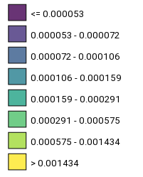
- legend2Image(legend, size=1, clipdimension=999, width=300, fontweight=400, fontsize=9, textcolor='black')
Given as input a legend returned by a call to one of the methods:
legendSingle(),legendCategories()orlegendGraduated(), this function returns an PILLOW image containing all the items of the legend.- Parameters:
legend (list of dicts) – Legend returned by one of the three methods to build a legend.
size (int, optional) – Size of the image to create, in the range [1,3] for “small” (30x30 pixels), “medium” (80x80 pixels) and “big” (256x256 pixels) dimensions. Default is 1.
clipdimension (int, optional) – Optional dimension of the square in pixel to be used to clip the output image to a smaller dimension (default is 999).
width (int, optional) – Width in pixels of the image (default is 300).
fontweight (int, optional) – Weight of the font used to display the descriptions of the legend items (default is 400, meaning plain text, use 300 for a thinner font, 600 or above for a bold font).
fontsize (int, optional) – Height in pixels of the font used to display the descriptions of the legend items (default is 9).
textcolor (str, optional) – Color of the text (default is ‘black’).
Example
Display a legend as a PILLOW image:
# Import libraries
from IPython.display import display
from geolayer import vectorlayer
import plotly.express as px

# Create a vectorlayer instance from a file dataset (geopackage)
vlayer = vectorlayer.file('.../EuroGlobalMap.gpkg', layer='CoastA', epsg=4258)

# Define a parametrical symbol
symbol = [
            [
               ["PolygonSymbolizer", "fill", 'FILL-COLOR'],
               ["PolygonSymbolizer", "fill-opacity", 0.8],
               ["LineSymbolizer", "stroke", "#000000"],
               ["LineSymbolizer", "stroke-width", 1.0]
            ]
]

# Create a graduated legend with 8 classes on the Shape_Area field
legend = vlayer.legendGraduated('Shape_Area',
                                px.colors.sequential.Viridis,
                                symbol=symbol,
                                interpolate=True,
                                classifier_name='Quantiles',
                                classifier_param1=8,
                                digits=6)

# Display the legend as an image
img = vlayer.legend2Image(legend, size=1, fontsize=13, fontweight=400, width=400)
display(img)
- legend2List(legend, title='', size=1, disabled=False, onclick=None)
Given as input a legend returned by a call to one of the methods:
legendSingle(),legendCategories()orlegendGraduated(), this function returns a clickable ipyvuetify List widget containing all the items of the legend.- Parameters:
legend (list of dicts) – Legend returned by one of the three methods to build a legend.
title (str, optional) – Title of the legend (default is ‘’).
size (int, optional) – Size of the image to create, in the range [1,3] for “small” (30x30 pixels), “medium” (80x80 pixels) and “big” (256x256 pixels) dimensions. Default is 1.
disabled (bool, optional) – If True, the
onclick (callable, optional) – Python function to call when the user clicks on one of the items of the List widget (default is None). The function must manage three parameters: widget, event, data. By accessing widgets.value the function can understand on which item the click event occurred (from 0 to nitems-1).
Example
Display a legend as a ipyvuetify List widget:
# Import libraries
from IPython.display import display
from geolayer import vectorlayer
import plotly.express as px

# Create a vectorlayer instance from a file dataset (geopackage)
vlayer = vectorlayer.file('.../EuroGlobalMap.gpkg', layer='CoastA', epsg=4258)

# Define a parametrical symbol
symbol = [
            [
               ["PolygonSymbolizer", "fill", 'FILL-COLOR'],
               ["PolygonSymbolizer", "fill-opacity", 0.8],
               ["LineSymbolizer", "stroke", "#000000"],
               ["LineSymbolizer", "stroke-width", 1.0]
            ]
]

# Create a graduated legend with 8 classes on the Shape_Area field
legend = vlayer.legendGraduated('Shape_Area',
                                px.colors.sequential.Viridis,
                                symbol=symbol,
                                interpolate=True,
                                classifier_name='Quantiles',
                                classifier_param1=8,
                                digits=6)

# Callback to be called when the user clicks on an item of the legend
def onclick(widget, event, data):
    print(legend[widget.value])

# Create a List widget from the legend
w = vlayer.legend2List(legend, title='Legend', size=2, onclick=onclick)
display(w)

- static symbolChange(symbol, color='#ff0000', fillColor='#ff0000', fillOpacity=1.0, strokeColor='#ffff00', strokeWidth=0.5, scalemin=None, scalemax=None, size_multiplier=1.0)
Change color and other properties of a parametric (i.e. generic) symbol and returns the modified symbol.
These tags can be used inside a symbol definition for creating a parametric symbol that can then be instantiated using these substitutions:
COLOR (parameter color)
FILL-COLOR (parameter fillColor)
FILL-OPACITY (parameter fillOpacity)
STROKE-COLOR (parameter strokeColor)
STROKE-WIDTH (parameter strokeWidth)
SCALE-MIN (parameter scalemin)
SCALE-MAX (parameter scalemax)
- Parameters:
symbol (list of lists, optional) – Symbol to be used for the rendering of the features. See the chapter Display vector datasets for a guide on how symbols are defined and the chapter Create symbols for vector datasets for help on the visual Symbol Editor.
color (str, optional) – Color to be substituted to the tag COLOR (default is ‘#ff0000’).
fillColor (str, optional) – Color to be substituted to the tag FILL-COLOR (default is ‘#ff0000’).
fillOpacity (float, optional) – Opacity value in [0,1] range to be substituted to the tag FILL-OPACITY (default is 1.0).
strokeColor (str, optional) – Color to be substituted to the tag STROKE-COLOR (default is ‘#ffff00’).
strokeWidth (float, optional) – Width of the stroke in pixels to be substituted to the tag STROKE-WIDTH (default is 0.5).
scalemin (float, optional) – Minimum scale denominator to be substituted to the tag SCALE-MIN to limit the zoom levels for which the symbol is visible (default is None).
scalemax (float, optional) – Maximum scale denominator to be substituted to the tag SCALE-MAX to limit the zoom levels for which the symbol is visible (default is None).
size_multiplier (float, optional) – Multiplier factor to be used for increasing/decreasing the size of markers of the width of strokes (default is 1.0).
- Returns:
modified_symbol – The input symbol modified by substituting the tags with the input parameter values.
- Return type:
list of lists
Example
Create and instantiate a parametric symbol:
# Import libraries
from geolayer import vectorlayer

# Define a parametric symbol (FILL-COLOR to be substituted with the actual color)
symbol = [
            [
               ["PolygonSymbolizer", "fill", 'FILL-COLOR'],
               ["PolygonSymbolizer", "fill-opacity", 0.8],
               ["LineSymbolizer", "stroke", "#000000"],
               ["LineSymbolizer", "stroke-width", 1.0]
            ]
]

# Instantiate the parametric symbol by substituting the FILL-COLOR tag with 'red'
symbol_modified = vectorlayer.symbolChange(symbol, fillColor='red')
- print()
Prints a textual description of the class instance.
- identify(lon, lat, zoom)
Given in input a geographic coordinate and a zoom level, returns a string containing info on the attributes of the feature under the (lat,lon) position.
- Parameters:
- Returns:
res – The string containing the attribute names and values of the identified feature.
- Return type:
- property identify_fields
Get/Set the list of attributes to return on an identify operation (click on a vector feature).
- Returns:
list_of_attributes – Names of the attributes to return on an identify operation
- Return type:
Example
Programmatically change the list of attributes:
vlayer.identify_fields = ['attribute1', 'attribute2']
print(vlayer.identify_fields)
- property identify_width
Get/Set the width of the popup widget that opens when an identify operation is done on a feature of the vector layer.
- Returns:
width – Width in pixels or any other CSS units of the popup widget (default is ‘180px’)
- Return type:
Example
Programmatically change the width of the identify popup:
vlayer.identify_width = '3vw'
print(vlayer.identify_width)
- tileLayer(max_zoom=22)
Creates an ipyleaflet.TileLayer object from an instance of vectorlayer, to be added to a Map for display.
- Returns:
tlayer – Instance of ipyleaflet.TileLayer to be added to a Map
- Return type:
ipyleaflet.TileLayer
Example
Create an ipyleaflet.TileLayer instance:
# Import libraries
from IPython.display import display
import ipyleaflet
from geolayer import vectorlayer

# Create a vectorlayer instance
vlayer = vectorlayer.file(...)

# Create an ipyleaflet Map
m = ipyleaflet.Map()

# Add the layer to the map
m.add(vlayer.tileLayer())

# Display the map
display(m)
- vectorlayer.symbol2Image(symbol=[], size=1, feature='Point', clipdimension=999, showborder=False)
Convert a symbol into a Pillow image (to be used in legends, etc.).
- Parameters:
symbol (list of lists, optional) – Symbol to convert into a Pillow image. See the chapter Display vector datasets for a guide on how symbols are defined and the chapter Create symbols for vector datasets for help on the visual Symbol Editor.
size (int, optional) – Size of the image to create, in the range [1,3] for “small” (30x30 pixels), “medium” (80x80 pixels) and “big” (256x256 pixels) dimensions. Default is 1.
feature (str, optional) – Type of feature to display: Polygon, Point or Polyline (default is ‘Point’).
clipdimension (int, optional) – Optional dimension of the square in pixel to be used to clip the output image to a smaller dimension (default is 999).
showborder (bool, optional) – If True a thin border is added to the image (default is False).
Example
Create a Pillow image from a symbol:
# Import libraries
from IPython.display import display
from geolayer.vectorlayer import symbol2Image

symbol = [
            [
                ["PolygonSymbolizer", "fill", 'yellow'],
                ["PolygonSymbolizer", "fill-opacity", 0.2],
                ["LineSymbolizer", "stroke", "#00ff00"],
                ["LineSymbolizer", "stroke-width", 4.0]
            ]
]

# Create the image
img = symbol2Image(symbol, feature='Polygon', size=2, showborder=True)

# Display the image
display(img)
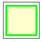
Image created by the example code above to convert a polygonal symbol to a Pillow image